Conditional Formatting Across An Entire Row In Google Sheets

I learned this from this post.

I always have students submit a contact sheet with their preferred email and ideally, a gmail account. Since students are different classes, I use conditional formatting to highlight entire rows based on responses and classes.

Step 1: Highlight the entire range that you want the conditional formatting to apply to. 

Make sure you select specific cells-- you may use A1:F (which highlights A1 to all of F):

Step 2: Under Format -> Conditional Formatting

Step 3:  A window will pop up on the side. The default is condition "Is Not Empty". 

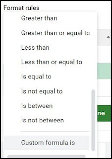
Step 4: Use the Drop down menu and scroll to the bottom to choose "Custom formula is"

Step 5: Enter the criteria you want; use the $ sign to lock your column reference: =$E1 = "text you want" IMPORTANT: It’s really important that the row here matches the first row of your highlighted range; for example if the range begins with Row 2, your range here must also be Row 2. In this example, my highlighted area begins with Row 1, so my formula also references Row 1 of the column in which I'm looking.

BTW, if you want to highlight rows containing a part of a word, I've found this works well: =SEARCH("your text",$C1) (again, the $C1 should be whatever row is the first row of your highlighted area).

That's it!